Stokes Classes
For spectropolarimetric data, the highest dimensionality object is the
StokesCube, which contains dimensions of (stokes, wavelength,
coord1, coord2), i.e. a map on the Sun of full Stokes profiles. In a
Jupyter notebook environment this multidimensional array can be fully
visualized by calling the plot() method:
>>> import stokespy
>>> stokes = stokespy.instload.load_HinodeSP_stokes(...)
>>> stokes.plot()
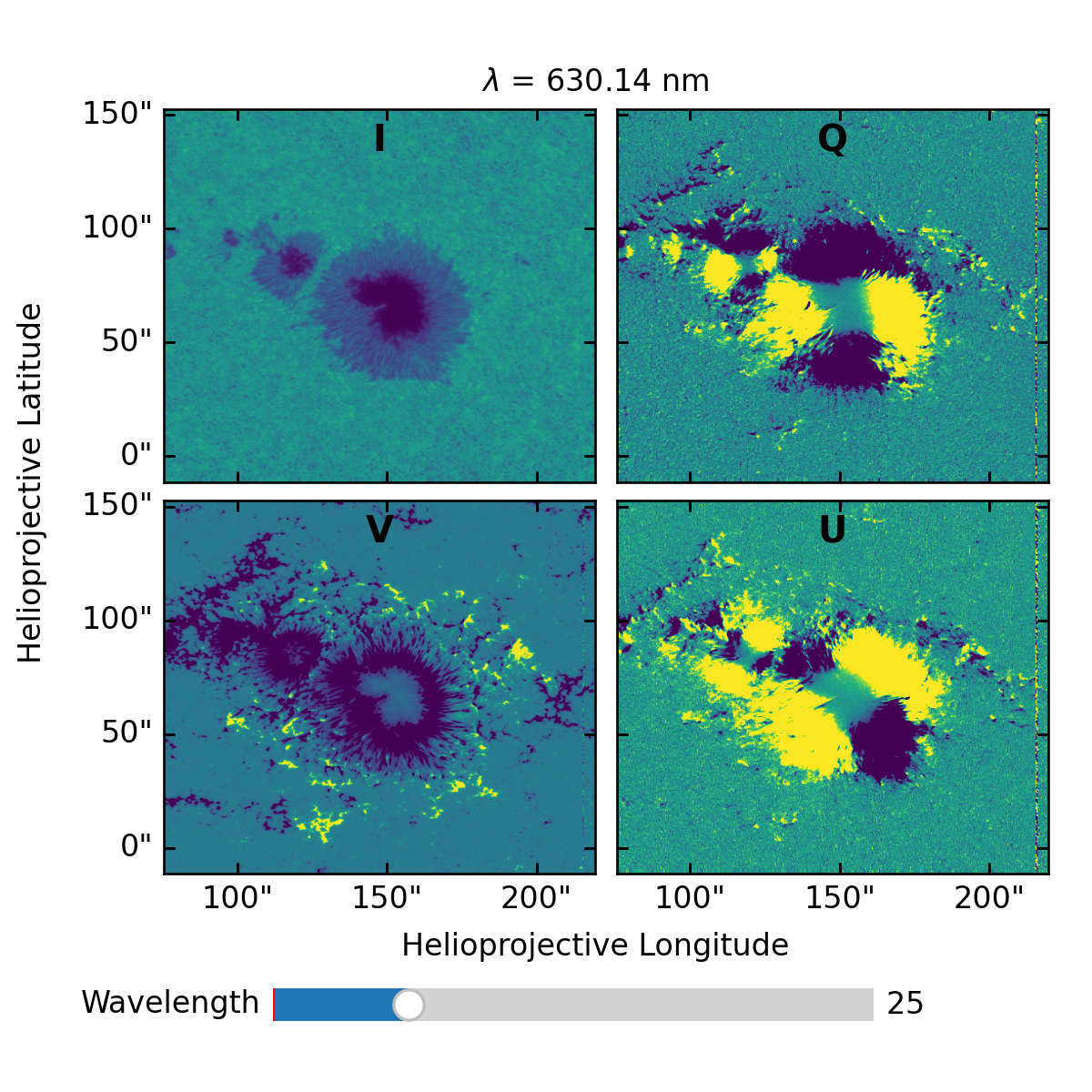
Here the wavelength slider allows one to scan the full Stokes data at each wavelength point.
Convenince methods for slicing give lower-dimensionality objects that can also be visualized, for example, for a map of only Stokes V:
>>> stokes.V.plot()
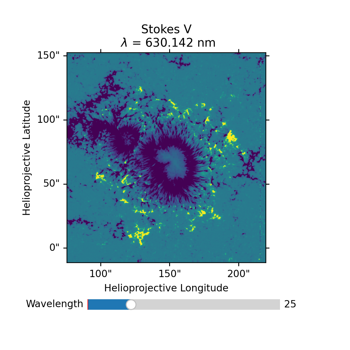
Here again the wavelength slider allows one to scan the data across wavelength.
A map at a single wavelength point can also be obtained:
>>> import astropy.units as u
>>> stokes.V_map(630.142 * u.nm).plot()
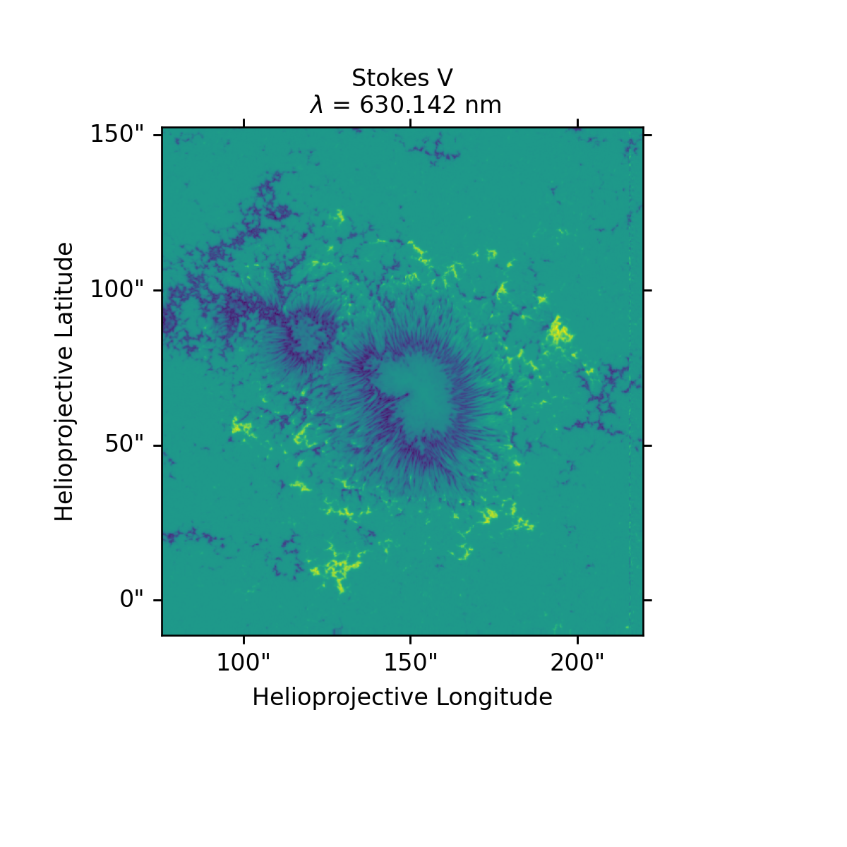
Notice how the wavelength was provided in physical units instead of an
index. The StokesCube world coordinate system (WCS) is
used to map physical (world) coordinates to array index, finding the
nearest valid index. In this way more general analysis code can be
written that supports arrays of various sizes, or sourced from
different instruments. If an integer is provided, it will be
interpreted as an index on the wavelength axis:
>>> stokes.V_map(25).plot()

In an analagous way, a line profile from any of the Stokes parameters can be obtained:
>>> coord = SkyCoord(Tx = 148 * u.arcsec, Ty = 67 * u.arcsec, frame = stokes.meta['frame'])
>>> stokes.V_profile(coord).plot()
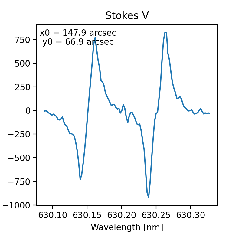
In this example the Stokes V profile from disk center is plotted.
Again, the advantage StokesPy provides is that this line of code will
provide the disk center profile for any valid StokesCube
object, regardless of its dimensionality or instrument of origin.
See the StokesCube API reference for the full set of
slicing access methods. Methods are also provided for common
polarimetric calculations, such as the total polarization with
P.